(Post exported from my old blog, now defunct -- published originally on July 12, 2010)
I just came back from SMBE2010, where I presented a poster about our recombination detection software and had the chance to see awesome research other people are doing. The poster can be downloaded here (1.MB in pdf format) and I'm distributing it under the Creative Commons License. Given the great feedback I got from other participants of the meeting, I thought it might be a good opportunity to comment about the work, guided by the poster figures. Please refer to the poster to follow the figures and the explanation, I'll try to reproduce here my presentation taking into account the commentaries I received.
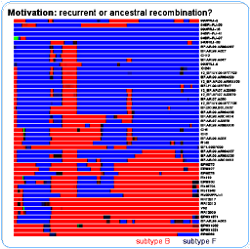
The motivation for the development of the model was to be able to say, for a given a mosaic structure, if the breakpoints can be explained by one recombination event or several. The recombination mosaic structure is usually inferred assuming the parental sequences (those not recombining) are known beforehand - in the figure they are the subtypes B and F - and recombination is then inferred when there is a change in the parental closest to the query sequence. Another problem is that it is common to analyze each one of the query sequences independently against the parentals - if all one wants is the "coloring", then this might be enough. For the above figure I analyzed each query sequence against one reference sequence from the subtypes B, F and C (thus comprising a quartet for each analysis). And we know that these mosaics don't tell the whole story.

If we know the topologies for both segments separated by the recombination breakpoint, then we can say, at least in theory, the minimum number of recombination events necessary to explain the difference (the real number can be much larger since we only detect those that lead to a change in the topology...). This minimum number is the Subtree Prune-and-Regraft distance, and is related to the problem of detection of horizontal gene transfers. In our case we devised an approximation to this distance based on the disagreement between all pairs of bipartitions belonging to the topologies: at each iteration we remove the smallest number of "leaves" such that the topologies will become more similar, and our approximate "uSPR distance" will be how many times we iterate this removal.
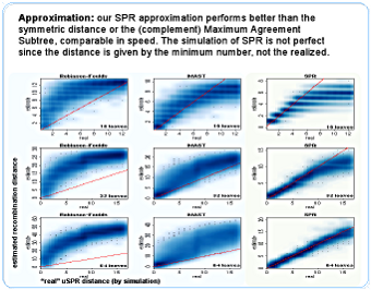
It is just an approximation, but it is better (closer to the SPR distance) than the Robinson-Foulds or the (complementary) Maximum Agreement Subtree distances, which compete in speed with our algorithm. For larger topologies it apparently works better than for smaller, but this is an artifact of the simulation - one realized SPR "neutralizes" previous ones, and it happens more often for small trees.
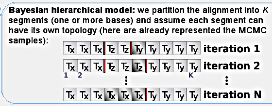
Our Bayesian model works with a partitioning of the alignment, where recombination can only occur between segments and never within. This doesn't pose a problem in practice since it will "shift" the recombinations to the border - the idea is that several neighboring breakpoints are equivalent to one breakpoint with a larger distance. This segments could be composed of one site each, but for computational reasons we usually set it up at five or ten base pairs. The drawback is the loss of hability to detect rate heterogeneity within the segment.
Each segment will have it own toplology (represented by Tx, Ty and Tz in the figure), which will coincide for many neighboring segments since we have the distance between them as a latent variable penalizing against too many breakpoints:
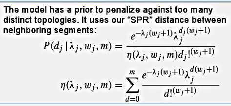
This is a truncated Poisson distribution, modified so that it can handle underdispersion - the parameter w will make the Poisson sharper around the mean - and each potential breakpoint has its own lambda and w.

The posterior distribution will have K terms for the segments (topology likelihood and evolutionary model priors) and K-1 terms for the potential breakpoints (distances between segments), as well as the hyper-priors. I use the term "potential breakpoint" because if two consecutive segments happen to have the same topology (distance equals zero) then we don't have an actual breakpoint. Again, considering only the recombinations that change the topology. This posterior distribution is calculated through MCMC sampling in the program called biomc2.
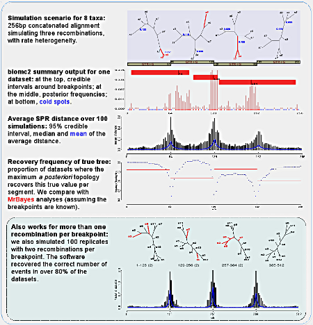
To test the algorithm, we did simulations with eight and twelve taxa datasets, simulating one (for the eight taxa datasets) or two recombinations per breakpoint. We present the output of the program biomc2.summarise, which interprets the posterior samples for one replicate: based on the posterior distribution of distances for each potential breakpoint, we neglect the actual distances and focus on whether it is larger than or equal to zero (second figure of the panel). Based on this multimodal distribution of breakpoints we infer the regions where no recombination was detected (that we call "cold spots"), credible intervals around each mode (red bars on top) or based on all values (red dots at bottom, together with the cold spots).
We also looked at the average distance for each potential breakpoint per replicate dataset, and show that indeed the software can correctly infer the location and amount of recombination for most replicates. It is worth remembering that we were generous in our simulations, in that there is still phylogenetic signal preserved on alignments with many mutations and a few recombinations. If recombination is much more frequent, then any two sites might represent distinct evolutionary histories and our method will fail.
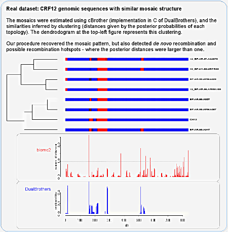
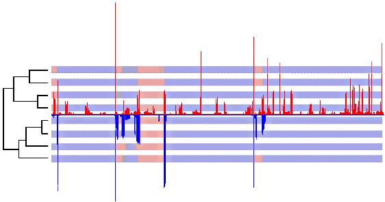
We then analyzed HIV genomic sequences with a very similar mosaic structure, as inferred by cBrother (an implementation of DualBrothers). Here it is important to say that we used cBrother only to estimate the mosaic structure of the recombinants, doing an independent analysis for each sequence against three reference parental sequences. Therefore the figure is not a direct comparison of the programs, contrary to what its unfortunate caption might induce us to think. The distinction is between analyzing all sequences at once or independently, in quartets of sequences. If we superpose the panels it might become clearer to compare them:
The curve in blue shows the positions where there is a change in closest parental for the query sequence, if each query sequence is analyzed neglecting the others. In red we have our algorithm estimating recombinations between all eleven sequences (eight query and three parental sequences). We can see that:
- all breakpoints detected by the independent analysis were also detected by our method;
- many recombinations were detected only when all sequences were analyzed at once, indicating that they do not involve the parental sequences - de novo recombination;
- if we look at the underlying topologies estimated by our method (figure S2 of the PLoS ONE paper), we see that those also detected by the independent analysis in fact involve the parentals while the others don't;
- biomc2 not only infers the location of recombination, but also its "strength" - given by the distance between topologies;

Finally, we show two further developments of the software: a point estimate for the recombination mosaic, and the relevance of the chosen prior over distances. The point estimate came from the need of a more easily interpretable summary of the distribution of breakpoints: instead of looking at the whole multimodal distribution, we may want to pay attention only to the peaks, or some other similar measure. This is a common problem in bioinformatics: to represent a collection of trees by a single one or to find a protein structure that represents best an ensemble of structures. In our case we have a collection of recombination mosaics (one per sample of the posterior distribution), and we elect the one with the smallest distance from all other mosaics - we had to devise a distance for this as well...
To show the importance of the prior distribution of distances, we compared it with simplified versions, like setting the penalty parameter w fixed at a low or high value. The overall behavior for all scenarios is lower resolution around breakpoints, and for weaker penalties we reconstruct the topologies better than for stronger ones, at the cost of inferring spurious breakpoints more often. We also compared the original model with a simplification where the topological distance is neglected and the prior considers only if the topologies are equal or not. This is similar to what cBrother and other programs do, and by looking at the top panel we observe that the results were also equivalent (blue lines labeled "cBrother" and "m=0"). In the same panel we plot the performance using our original ("unrestricted") model as a gray area.
I also submitted the poster to the F1000 Poster Bank.
References:
de Oliveira Martins, L., Leal, É., & Kishino, H. (2008). Phylogenetic Detection of Recombination with a Bayesian Prior on the Distance between Trees PLoS ONE, 3 (7) DOI: 10.1371/journal.pone.0002651
de Oliveira Martins, L., & Kishino, H. (2009). Distribution of distances between topologies and its effect on detection of phylogenetic recombination Annals of the Institute of Statistical Mathematics, 62 (1), 145-159 DOI: 10.1007/s10463-009-0259-8


No comments:
Post a Comment
Use the space below to ask, inform and criticize -- if you are not very happy please read the rules for commenting.
Please, do not include unrelated, commercial sites not even in your signature.